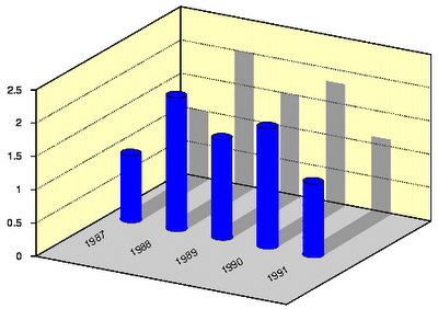
And now, let us see the code. We will assume that we want to plot the following set of data
1987 1
1988 2
1989 1.5
1990 1.8
1991 1.1
Now, here is the full code
reset
set border 0
unset key
unset colorbox
set cbrange [-0.1:2]
set isosample 10,10
set sample 100
set parametric
set ticslevel 0

a=2
b=0.5
c=-0.5
d=5.5
e=(c+d)/2.0
f=(d-c)
r=0.2

set multiplot
set urange [0:1]
set vrange [0:1]
set yrange [c:d]
set xrange [c:d]
set zrange [0:2.5]
unset xtics
unset ytics
set ztics out
set grid ztics

# First, we draw the 'box' around the plotting volume
set palette model RGB functions 0.8, 0.8,0.8
splot 10*u-0.5, c+f*v,0 w pm3d

set palette model RGB functions 1, 254.0/255.0, 189.0/255.0
splot -0.5, c+f*u, 2.5*v w pm3d , 10*u-0.5, d, 2.5*v w pm3d

set border 1+2+4+8+16+32+64+256+512
# Then we put on all the shadow. This step can be skipped
set palette model RGB functions 0.6,0.6,0.6
# First shadow, and so on
splot 2*r*u-1.5*r, d, v w pm3d,\
2*r*u-v/(d-e)*r-r, (d-e)*v+e, 0 w pm3d,\
2*r*u+1-1.5*r, d, 2*v w pm3d,\
2*r*u-v/(d-e)*r+1-r, (d-e)*v+e, 0 w pm3d,\
2*r*u+2-1.5*r, d, 1.5*v w pm3d,\
2*r*u-v/(d-e)*r+2-r, (d-e)*v+e, 0 w pm3d,\
2*r*u+3-1.5*r, d, 1.8*v w pm3d,\
2*r*u-v/(d-e)*r+3-r, (d-e)*v+e, 0 w pm3d,\
2*r*u+4-1.5*r, d, 1.1*v w pm3d,\
2*r*u-v/(d-e)*r+4-r, (d-e)*v+e, 0 w pm3d

set label 1 '1987' at 0, 0.6, 0 rotate by 30
set label 2 '1988' at 1, 0.6, 0 rotate by 30
set label 3 '1989' at 2, 0.6, 0 rotate by 30
set label 4 '1990' at 3, 0.6, 0 rotate by 30
set label 5 '1991' at 4, 0.6, 0 rotate by 30

set palette model RGB functions 0, 0, 1
f(u, xx) = r*cos(2*u*pi)+xx
g(u, yy) = r*sin(2*u*pi)+yy
splot f(u,0), g(u,e), 0 w l lt -1 lw a, f(u,0),g(u,e),v w pm3d, f(u,0), g(u,e),1 w l lt -1 lw b,\
f(u,1), g(u,e), 0 w l lt -1 lw a, f(u,1),g(u,e),2*v w pm3d, f(u,1), g(u,e), 2 w l lt -1 lw b,\
f(u,2), g(u,e), 0 w l lt -1 lw a, f(u,2),g(u,e),1.5*v w pm3d, f(u,2), g(u,e), 1.5 w l lt -1 lw b,\
f(u,3), g(u,e), 0 w l lt -1 lw a, f(u,3),g(u,e),1.8*v w pm3d, f(u,3), g(u,e), 1.8 w l lt -1 lw b,\
f(u,4), g(u,e), 0 w l lt -1 lw a, f(u,4),g(u,e),1.1*v w pm3d, f(u,4), g(u,e), 1.1 w l lt -1 lw b
unset multiplot
The first part of the code is just general setup, which determines how our figure will be scaled. The only thing to watch out for is the definitions of a, b... f. These are needed, because otherwise the aspect ratio of the cylinders would change, and they would be elongated along one (probably the y) axis. Therefore, it is essential to set the xrange and yrange to the same value.
In the figure, the actual graph has a background, which is yellow for the vertical planes, and gray for the horizontal one. We add these as separate plots in a multiplot command. So,
reset
...
set parametric
...
set urange [0:1]
set vrange [0:1]
...
# First, we draw the 'box' around the plotting volume
set palette model RGB functions 0.8, 0.8,0.8
splot 10*u-0.5, c+f*v,0 w pm3d

set palette model RGB functions 1, 254.0/255.0, 189.0/255.0
splot -0.5, c+f*u, 2.5*v w pm3d , 10*u-0.5, d, 2.5*v w pm3d
plots three planes, below, behind and next to the graph. I would point out that we used parametric plot, which we defined with 'set parametric' and the 'set urange', 'set vrange' commands. The second point of interest is the colouring of the planes: we do this by setting a palette, which contains only one colour, e.g., light gray,
set palette model RGB functions 0.8, 0.8,0.8
or
set palette model RGB functions 1, 254.0/255.0, 189.0/255.0
The next step is to plot the shadows of the bars. This is done by drawing rectangles of the proper size on the back plane, and also, by drawing parallelograms on the horizontal plane. These are drawn in a slightly darker shade of gray, so we have got to re-define our palette.
Once we are done with the shadows, we set the labels, which will just be the values of the first column in our data file. We have got to rotate the labels by 30 degrees, so that they will be parallel to the edge of our box.
Finally, we have got to plot the bars themselves. First, we choose a colour for them, blue in this case, and set the palette accordingly. If we simply plotted cylinders using 'pm3d', we wouldn't have edges, or we would have too many. In order to avoid this situation, we put on the two rims of the cylinder by hand. This is why each cylinder consists of actually three plots: the bottom, the surface and the top. Note that the cylinders are open, they only look closed because we can't see to the bottom of them. This means that you have got to be a bit careful when setting the 'view' (which we didn't do here, we simply took the default value of 60,30).
There you have the shaded 3D bars.
If you are using gnuplot, I assume that you also use Linux. If that's the case, this whole procedure can easily be scripted, so then you wouldn't have to set everything by hand. I might post a possible implementation sometime later.
Hi!
ReplyDeleteHere is a problem for the future:
I've a hole pattern of a bolted flange
Resulting from FEA I've calculated the screw loads acting at every screw.
Now I want to have a picture of bars, each bar corresponding to one screw.
Every bar shall be located at the position of one screw, the height shall correspond to the screw load.
My input-date file has one row for every screw with 3 values: x-Position, y-Position, screw load.
I tried OpenOffice Calc, mathcad and gnuplot, but have had no sucess.
I think the solution shown here is very close to my problem.
Greetings from Germany